R Tutorial |
|
| R Tutorial❮ Home Next ❯ Learn RR is a programming language. R is often used for statistical computing and graphical presentation to analyze and visualize data. Start learning R now »
Examples in Each ChapterWith our "Try it Yourself" editor, you can edit R code and view the result. ExampleHow to output some text, and how to do a simple calculation in R: "Hello World!" 5 + 5 Result: [1] "Hello World!" [1] 10 Try it Yourself » ExampleHow you can use R to easily create a graph with numbers from 1 to 10 on both the x and y axis: plot(1:10) Result: 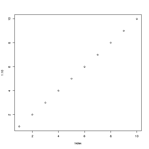
Try it Yourself » We recommend reading this tutorial, in the sequence listed in the left menu.
R ExercisesTest Yourself With ExercisesExercise:Insert the missing part of the code below to output "Hello World". Hello World
Submit Answer » Start the Exercise
My LearningTrack your progress with the free "My Learning" program here at W3Schools. Log in to your account, and start earning points! This is an optional feature. You can study at W3Schools without using My Learning. 
R ExamplesLearn by examples! This tutorial supplements all explanations with clarifying examples. See All R Examples
R QuizLearn by taking a quiz! This quiz will give you a signal of how much you know about R. Take the R Quiz
|
| R IntroductionWhat is RR is a popular programming language used for statistical computing and graphical presentation. Its most common use is to analyze and visualize data.
Why Use R?- It is a great resource for data analysis, data visualization, data science and machine learning
- It provides many statistical techniques (such as statistical tests, classification, clustering and data reduction)
- It is easy to draw graphs in R, like pie charts, histograms, box plot, scatter plot, etc++
- It works on different platforms (Windows, Mac, Linux)
- It is open-source and free
- It has a large community support
- It has many packages (libraries of functions) that can be used to solve different problems
Get StartedThis tutorial will teach you the basics of R. It is not necessary to have any prior programming experience. Get Started Now » |
| R Get Started❮ Previous Next ❯
How to Install RTo install R, go to https://cloud.r-project.org/ and download the latest version of R for Windows, Mac or Linux. When you have downloaded and installed R, you can run R on your computer. The screenshot below shows how it may look like when you run R on a Windows PC: 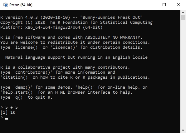
If you type 5 + 5, and press enter, you will see that R outputs 10.
Learning R at W3SchoolsWhen learning R at W3Schools.com, you can use our "Try it Yourself" tool, which shows both the code and the result in your browser. This will make it easier for you to test and understand every part as we move forward: Example5 + 5 Result: [1] 10 Try it Yourself »
|
| R Syntax❮ Previous Next ❯
SyntaxTo output text in R, use single or double quotes: Example"Hello World!" Try it Yourself » To output numbers, just type the number (without quotes): Example5 10 25 Try it Yourself » To do simple calculations, add numbers together: Example5 + 5 Try it Yourself » Congratulations! You have now written your first R code. |
R Print Output❮ Previous Next ❯
PrintUnlike many other programming languages, you can output code in R without using a print function: Example"Hello World!" Try it Yourself » However, R does have a print() function available if you want to use it. This might be useful if you are familiar with other programming languages, such as Python, which often uses the print() function to output code. Exampleprint("Hello World!") Try it Yourself » And there are times you must use the print() function to output code, for example when working with for loops (which you will learn more about in a later chapter): Examplefor (x in 1:10) { print(x) } Try it Yourself » Conclusion: It is up to you whether you want to use the print() function to output code. However, when your code is inside an R expression (e.g. inside curly braces {} like in the example above), use the print() function to output the result.
|
| R Comments❮ Previous Next ❯
CommentsComments can be used to explain R code, and to make it more readable. It can also be used to prevent execution when testing alternative code. Comments starts with a #. When executing code, R will ignore anything that starts with #. This example uses a comment before a line of code: Example# This is a comment "Hello World!" Try it Yourself » This example uses a comment at the end of a line of code: Example"Hello World!" # This is a comment Try it Yourself » Comments does not have to be text to explain the code, it can also be used to prevent R from executing the code: Example# "Good morning!" "Good night!" Try it Yourself »
Multiline CommentsUnlike other programming languages, such as Java, there are no syntax in R for multiline comments. However, we can just insert a # for each line to create multiline comments: Example# This is a comment # written in # more than just one line "Hello World!" Try it Yourself »
❮ Previous Next ❯
|
| R Variables❮ Previous Next ❯
Creating Variables in RVariables are containers for storing data values. R does not have a command for declaring a variable. A variable is created the moment you first assign a value to it. To assign a value to a variable, use the <- sign. To output (or print) the variable value, just type the variable name: Examplename <- "John" age <- 40
name # output "John" age # output 40 Try it Yourself » From the example above, name and age are variables, while "John" and 40 are values. In other programming language, it is common to use = as an assignment operator. In R, we can use both = and <- as assignment operators. However, <- is preferred in most cases because the = operator can be forbidden in some contexts in R.
Print / Output VariablesCompared to many other programming languages, you do not have to use a function to print/output variables in R. You can just type the name of the variable: Examplename <- "John Doe"
name # auto-print the value of the name variable Try it Yourself » However, R does have a print() function available if you want to use it. This might be useful if you are familiar with other programming languages, such as Python, which often use a print() function to output variables. Examplename <- "John Doe"
print(name) # print the value of the name variable Try it Yourself » And there are times you must use the print() function to output code, for example when working with for loops (which you will learn more about in a later chapter): Examplefor (x in 1:10) { print(x) } Try it Yourself » Conclusion: It is up to your if you want to use the print() function or not to output code. However, when your code is inside an R expression (for example inside curly braces {} like in the example above), use the print() function if you want to output the result.
❮ Previous Next ❯
|
R Concatenate Elements
Concatenate ElementsYou can also concatenate, or join, two or more elements, by using the paste() function.To combine both text and a variable, R uses comma (,):Exampletext <- "awesome"
paste("R is", text)You can also use , to add a variable to another variable:Exampletext1 <- "R is"text2 <- "awesome"
paste(text1, text2)For numbers, the + character works as a mathematical operator:Examplenum1 <- 5num2 <- 10
num1 + num2If you try to combine a string (text) and a number, R will give you an error:Examplenum <- 5text <- "Some text"
num + textResult:Error in num + text : non-numeric argument to binary operator |
R Multiple Variables
Multiple VariablesR allows you to assign the same value to multiple variables in one line:Example# Assign the same value to multiple variables in one linevar1 <- var2 <- var3 <- "Orange"
# Print variable valuesvar1var2var3
|
R Variable Names (Identifiers)
Variable NamesA variable can have a short name (like x and y) or a more descriptive name (age, carname, total_volume). Rules for R variables are:A variable name must start with a letter and can be a combination of letters, digits, period(.)
and underscore(_). If it starts with period(.), it cannot be followed by a digit.A variable name cannot start with a number or underscore (_)Variable names are case-sensitive (age, Age and AGE are three different variables)Reserved words cannot be used as variables (TRUE, FALSE, NULL, if...)
# Legal variable names:myvar <- "John"my_var <- "John"myVar <- "John"MYVAR <- "John"myvar2 <- "John".myvar <- "John"
# Illegal variable names:2myvar <- "John"my-var <- "John"my var <- "John"_my_var <- "John"my_v@ar <- "John"TRUE <- "John"Remember that variable names are case-sensitive!
|
| R Data Types❮ Previous Next ❯
Data TypesIn programming, data type is an important concept. Variables can store data of different types, and different types can do different things. In R, variables do not need to be declared with any particular type, and can even change type after they have been set: Examplemy_var <- 30 # my_var is type of numeric my_var <- "Sally" # my_var is now of type character (aka string) Try it Yourself » R has a variety of data types and object classes. You will learn much more about these as you continue to get to know R.
Basic Data TypesBasic data types in R can be divided into the following types: - numeric - (10.5, 55, 787)
- integer - (1L, 55L, 100L, where the letter "L" declares this as an integer)
- complex - (9 + 3i, where "i" is the imaginary part)
- character (a.k.a. string) - ("k", "R is exciting", "FALSE", "11.5")
- logical (a.k.a. boolean) - (TRUE or FALSE)
We can use the class() function to check the data type of a variable: Example# numeric x <- 10.5 class(x)
# integer x <- 1000L class(x)
# complex x <- 9i + 3 class(x)
# character/string x <- "R is exciting" class(x)
# logical/boolean x <- TRUE class(x) Try it Yourself » You will learn much more about the individual data types in the upcoming chapters.
|
| R Numbers❮ Previous Next ❯
NumbersThere are three number types in R: Variables of number types are created when you assign a value to them: Examplex <- 10.5 # numeric y <- 10L # integer z <- 1i # complex
NumericA numeric data type is the most common type in R, and contains any number with or without a decimal, like: 10.5, 55, 787: Examplex <- 10.5 y <- 55
# Print values of x and y x y
# Print the class name of x and y class(x) class(y) Try it Yourself »
IntegerIntegers are numeric data without decimals. This is used when you are certain that you will never create a variable that should contain decimals. To create an integer variable, you must use the letter L after the integer value: Examplex <- 1000L y <- 55L
# Print values of x and y x y
# Print the class name of x and y class(x) class(y) Try it Yourself »
ComplexA complex number is written with an "i" as the imaginary part: Examplex <- 3+5i y <- 5i
# Print values of x and y x y
# Print the class name of x and y class(x) class(y) Try it Yourself »
Type ConversionYou can convert from one type to another with the following functions: - as.numeric()
- as.integer()
- as.complex()
Examplex <- 1L # integer y <- 2 # numeric
# convert from integer to numeric: a <- as.numeric(x)
# convert from numeric to integer: b <- as.integer(y)
# print values of x and y x y
# print the class name of a and b class(a) class(b) Try it Yourself »
|
| R Math❮ Previous Next ❯
Simple MathIn R, you can use operators to perform common mathematical operations on numbers. The + operator is used to add together two values: Example10 + 5 Try it Yourself » And the - operator is used for subtraction: Example10 - 5 Try it Yourself » You will learn more about available operators in our R Operators Tutorial.
Built-in Math FunctionsR also has many built-in math functions that allows you to perform mathematical tasks on numbers. For example, the min() and max() functions can be used to find the lowest or highest number in a set: Examplemax(5, 10, 15)
min(5, 10, 15) Try it Yourself »
sqrt()The sqrt() function returns the square root of a number: Examplesqrt(16) Try it Yourself »
abs()The abs() function returns the absolute (positive) value of a number: Exampleabs(-4.7) Try it Yourself »
ceiling() and floor()The ceiling() function rounds a number upwards to its nearest integer, and the floor() function rounds a number downwards to its nearest integer, and returns the result: Exampleceiling(1.4)
floor(1.4) Try it Yourself »
❮ Previous Next ❯
|
| R Strings❮ Previous Next ❯
String LiteralsStrings are used for storing text. A string is surrounded by either single quotation marks, or double quotation marks: "hello" is the same as 'hello': Example"hello" 'hello' Try it Yourself »
Assign a String to a VariableAssigning a string to a variable is done with the variable followed by the <- operator and the string: Examplestr <- "Hello" str # print the value of str Try it Yourself »
Multiline StringsYou can assign a multiline string to a variable like this: Examplestr <- "Lorem ipsum dolor sit amet, consectetur adipiscing elit, sed do eiusmod tempor incididunt ut labore et dolore magna aliqua."
str # print the value of str Try it Yourself » However, note that R will add a "\n" at the end of each line break. This is called an escape character, and the n character indicates a new line. If you want the line breaks to be inserted at the same position as in the code, use the cat() function: Examplestr <- "Lorem ipsum dolor sit amet, consectetur adipiscing elit, sed do eiusmod tempor incididunt ut labore et dolore magna aliqua."
cat(str) Try it Yourself »
String LengthThere are many useful string functions in R. For example, to find the number of characters in a string, use the nchar() function: Examplestr <- "Hello World!"
nchar(str) Try it Yourself »
Check a StringUse the grepl() function to check if a character or a sequence of characters are present in a string: Examplestr <- "Hello World!"
grepl("H", str) grepl("Hello", str) grepl("X", str) Try it Yourself »
Combine Two StringsUse the paste() function to merge/concatenate two strings: Examplestr1 <- "Hello" str2 <- "World"
paste(str1, str2) Try it Yourself »
|
R Escape Characters
Escape CharactersTo insert characters that are illegal in a string, you must use an escape character.An escape character is a backslash \ followed by the character you want to insert.An example of an illegal character is a double quote inside a string that is surrounded by double quotes:Examplestr <- "We are the so-called "Vikings", from the north."
strResult:Error: unexpected symbol in "str <- "We are the so-called "Vikings"To fix this problem, use the escape character \":ExampleThe escape character allows you to use double quotes when you normally would not be allowed:str <- "We are the so-called \"Vikings\", from the north."
strcat(str)Note that auto-printing the str variable will print the backslash in the output. You can use the cat() function to print it without backslash.Other escape characters in R:Code | Result | \\ | Backslash | \n | New Line | \r | Carriage Return | \t | Tab | \b | Backspace |
|
| R Booleans / Logical Values❮ Previous Next ❯
Booleans (Logical Values)In programming, you often need to know if an expression is true or false. You can evaluate any expression in R, and get one of two answers, TRUE or FALSE. When you compare two values, the expression is evaluated and R returns the logical answer: Example10 > 9 # TRUE because 10 is greater than 9 10 == 9 # FALSE because 10 is not equal to 9 10 < 9 # FALSE because 10 is greater than 9 Try it Yourself » You can also compare two variables: Examplea <- 10 b <- 9
a > b Try it Yourself » You can also run a condition in an if statement, which you will learn much more about in the if..else chapter. Examplea <- 200 b <- 33
if (b > a) { print ("b is greater than a") } else { print("b is not greater than a")
} Try it Yourself » |
| R Operators❮ Previous Next ❯
OperatorsOperators are used to perform operations on variables and values. In the example below, we use the + operator to add together two values: Example10 + 5 Try it Yourself » R divides the operators in the following groups: - Arithmetic operators
- Assignment operators
- Comparison operators
- Logical operators
- Miscellaneous operators
R Arithmetic OperatorsArithmetic operators are used with numeric values to perform common mathematical operations:
R Assignment OperatorsAssignment operators are used to assign values to variables: Examplemy_var <- 3
my_var <<- 3
3 -> my_var
3 ->> my_var
my_var # print my_var Try it Yourself » Note: <<- is a global assigner. You will learn more about this in the Global Variable chapter. It is also possible to turn the direction of the assignment operator. x <- 3 is equal to 3 -> x
R Comparison OperatorsComparison operators are used to compare two values:
R Logical OperatorsLogical operators are used to combine conditional statements: Operator | Description | & | Element-wise Logical AND operator. Returns TRUE if both elements are TRUE | && | Logical AND operator - Returns TRUE if both statements are TRUE | | | Elementwise- Logical OR operator. Returns TRUE if one of the statements is TRUE | || | Logical OR operator. Returns TRUE if one of the statements is TRUE | ! | Logical NOT - Returns FALSE if statement is TRUE |
R Miscellaneous OperatorsMiscellaneous operators are used to manipulate data: Operator | Description | Example | : | Creates a series of numbers in a sequence | x <- 1:10 | %in% | Find out if an element belongs to a vector | x %in% y | %*% | Matrix Multiplication | x <- Matrix1 %*% Matrix2 |
Note: You will learn more about Matrix multiplication and matrices in a later chapter.
❮ Previous Next ❯ |
| R If ... Else❮ Previous Next ❯
Conditions and If StatementsR supports the usual logical conditions from mathematics: These conditions can be used in several ways, most commonly in "if statements" and loops.
The if StatementAn "if statement" is written with the if keyword, and it is used to specify a block of code to be executed if a condition is TRUE: Examplea <- 33 b <- 200
if (b > a) { print("b is greater than a") } Try it Yourself » In this example we use two variables, a and b, which are used as a part of the if statement to test whether b is greater than a. As a is 33, and b is 200, we know that 200 is greater than 33, and so we print to screen that "b is greater than a". R uses curly brackets { } to define the scope in the code.
Else IfThe else if keyword is R's way of saying "if the previous conditions were not true, then try this condition": Examplea <- 33 b <- 33
if (b > a) { print("b is greater than a") } else if (a == b) { print ("a and b are equal") } Try it Yourself » In this example a is equal to b, so the first condition is not true, but the else if condition is true, so we print to screen that "a and b are equal". You can use as many else if statements as you want in R.
If ElseThe else keyword catches anything which isn't caught by the preceding conditions: Examplea <- 200 b <- 33
if (b > a) { print("b is greater than a") } else if (a == b) { print("a and b are equal") } else { print("a is greater than b") } Try it Yourself » In this example, a is greater than b, so the first condition is not true, also the else if condition is not true, so we go to the else condition and print to screen that "a is greater than b". You can also use else without else if: Examplea <- 200 b <- 33
if (b > a) { print("b is greater than a") } else { print("b is not greater than a") } Try it Yourself »
❮ Previous Next ❯ |
R Nested If
Nested If StatementsYou can also have if statements inside if statements, this is called nested if statements.Examplex <- 41
if (x > 10) { print("Above ten") if (x > 20) { print("and also above 20!") } else { print("but not above 20.") }} else { print("below 10.")}
|
R - AND OR Operators❮ Previous Next ❯
ANDThe & symbol (and) is a logical operator, and is used to combine conditional statements: ExampleTest if a is greater than b, AND if c is greater than a: a <- 200 b <- 33 c <- 500
if (a > b & c > a) { print("Both conditions are true") } Try it Yourself »
ORThe | symbol (or) is a logical operator, and is used to combine conditional statements: ExampleTest if a is greater than b, or if c is greater than a: a <- 200 b <- 33 c <- 500
if (a > b | a > c) { print("At least one of the conditions is true") } Try it Yourself »
❮ Previous Next ❯
|
| R While Loop
LoopsLoops can execute a block of code as long as a specified condition is reached.Loops are handy because they save time, reduce errors, and they make code more readable.R has two loop commands:
R While LoopsWith the while loop we can execute a set of statements as long as a condition is TRUE:ExamplePrint i as long as i is less than 6:i <- 1while (i < 6) { print(i) i <- i + 1}In the example above, the loop will continue to produce numbers ranging from 1 to 5. The loop will stop at 6 because 6 < 6 is FALSE.The while loop requires relevant variables to be ready, in this example we need to define an indexing variable, i, which we set to 1.Note: remember to increment i, or else the loop will continue forever.
BreakWith the break statement, we can stop the loop even if the while condition is TRUE:ExampleExit the loop if i is equal to 4.i <- 1while (i < 6) { print(i) i <- i + 1 if (i == 4) { break }}The loop will stop at 3 because we have chosen to finish the loop by using the break statement when i is equal to 4 (i == 4).
NextWith the next statement, we can skip an iteration without terminating the loop:ExampleSkip the value of 3:i <- 0while (i < 6) { i <- i + 1 if (i == 3) { next } print(i)}When the loop passes the value 3, it will skip it and continue to loop.
Yahtzee!If .. Else Combined with a While LoopTo demonstrate a practical example, let us say we play a game of Yahtzee!ExamplePrint "Yahtzee!" If the dice number is 6:dice <- 1while (dice <= 6) { if (dice < 6) { print("No Yahtzee") } else { print("Yahtzee!") } dice <- dice + 1}If the loop passes the values ranging from 1 to 5, it prints "No Yahtzee". Whenever it passes the value 6, it prints "Yahtzee!". |
| R For Loop❮ Previous Next ❯
For LoopsA for loop is used for iterating over a sequence: Examplefor (x in 1:10) { print(x) } Try it Yourself » This is less like the for keyword in other programming languages, and works more like an iterator method as found in other object-oriented programming languages. With the for loop we can execute a set of statements, once for each item in a vector, array, list, etc.. You will learn about lists and vectors, etc in a later chapter. ExamplePrint every item in a list: fruits <- list("apple", "banana", "cherry")
for (x in fruits) { print(x) } Try it Yourself » ExamplePrint the number of dices: dice <- c(1, 2, 3, 4, 5, 6)
for (x in dice) { print(x) } Try it Yourself » The for loop does not require an indexing variable to set beforehand, like with while loops.
BreakWith the break statement, we can stop the loop before it has looped through all the items: ExampleStop the loop at "cherry": fruits <- list("apple", "banana", "cherry")
for (x in fruits) { if (x == "cherry") { break } print(x) } Try it Yourself » The loop will stop at "cherry" because we have chosen to finish the loop by using the break statement when x is equal to "cherry" (x == "cherry").
NextWith the next statement, we can skip an iteration without terminating the loop: ExampleSkip "banana": fruits <- list("apple", "banana", "cherry")
for (x in fruits) { if (x == "banana") { next } print(x) } Try it Yourself » When the loop passes "banana", it will skip it and continue to loop.
Yahtzee!If .. Else Combined with a For LoopTo demonstrate a practical example, let us say we play a game of Yahtzee! ExamplePrint "Yahtzee!" If the dice number is 6: dice <- 1:6
for(x in dice) { if (x == 6) { print(paste("The dice number is", x, "Yahtzee!")) } else { print(paste("The dice number is", x, "Not Yahtzee")) } } Try it Yourself » If the loop reaches the values ranging from 1 to 5, it prints "No Yahtzee" and its number. When it reaches the value 6, it prints "Yahtzee!" and its number.
❮ Previous Next ❯
|
R Nested Loops
Nested LoopsIt is also possible to place a loop inside another loop. This is called a nested loop:ExamplePrint the adjective of each fruit in a list:adj <- list("red", "big", "tasty")
fruits <- list("apple", "banana", "cherry") for (x in adj) { for (y in fruits) { print(paste(x, y)) }}
|
| R Functions❮ Previous Next ❯
A function is a block of code which only runs when it is called. You can pass data, known as parameters, into a function. A function can return data as a result.
Creating a FunctionTo create a function, use the function() keyword: Examplemy_function <- function() { # create a function with the name my_function print("Hello World!") }
Call a FunctionTo call a function, use the function name followed by parenthesis, like my_function(): Examplemy_function <- function() { print("Hello World!") }
my_function() # call the function named my_function Try it Yourself »
ArgumentsInformation can be passed into functions as arguments. Arguments are specified after the function name, inside the parentheses. You can add as many arguments as you want, just separate them with a comma. The following example has a function with one argument (fname). When the function is called, we pass along a first name, which is used inside the function to print the full name: Examplemy_function <- function(fname) { paste(fname, "Griffin") }
my_function("Peter") my_function("Lois") my_function("Stewie") Try it Yourself » Parameters or Arguments?The terms "parameter" and "argument" can be used for the same thing: information that are passed into a function. From a function's perspective: A parameter is the variable listed inside the parentheses in the function definition. An argument is the value that is sent to the function when it is called.
Number of ArgumentsBy default, a function must be called with the correct number of arguments. Meaning that if your function expects 2 arguments, you have to call the function with 2 arguments, not more, and not less: ExampleThis function expects 2 arguments, and gets 2 arguments: my_function <- function(fname, lname) { paste(fname, lname) }
my_function("Peter", "Griffin") Try it Yourself » If you try to call the function with 1 or 3 arguments, you will get an error: ExampleThis function expects 2 arguments, and gets 1 argument: my_function <- function(fname, lname) { paste(fname, lname) }
my_function("Peter") Try it Yourself »
Default Parameter ValueThe following example shows how to use a default parameter value. If we call the function without an argument, it uses the default value: Examplemy_function <- function(country = "Norway") { paste("I am from", country) }
my_function("Sweden") my_function("India") my_function() # will get the default value, which is Norway my_function("USA") Try it Yourself »
Return ValuesTo let a function return a result, use the return() function: Examplemy_function <- function(x) { return (5 * x) }
print(my_function(3)) print(my_function(5)) print(my_function(9)) Try it Yourself » The output of the code above will be: [1] 15 [1] 25 [1] 45
❮ Previous Next ❯ |
R Nested Functions
Nested FunctionsThere are two ways to create a nested function:Call a function within another function.Write a function within a function.
ExampleCall a function within another function:Nested_function <- function(x, y) { a <- x + y return(a)}
Nested_function(Nested_function(2,2), Nested_function(3,3))Example ExplainedThe function tells x to add y.The first input Nested_function(2,2) is "x" of the main function.The second input Nested_function(3,3) is "y" of the main function.The output is therefore (2+2) + (3+3) = 10.ExampleWrite a function within a function:Outer_func <- function(x) { Inner_func <- function(y) { a <- x + y return(a) } return (Inner_func)}output <- Outer_func(3) # To call the Outer_funcoutput(5)Example ExplainedYou cannot directly call the function because the Inner_func has been defined (nested) inside the Outer_func.We need to call Outer_func first in order to call Inner_func as a second step.We need to create a new variable called output and give it a value, which is 3 here.We then print the output with the desired value of "y", which in this case is 5.The output is therefore 8 (3 + 5).
|
R Function Recursion
RecursionR also accepts function recursion, which means a defined function can call itself.Recursion is a common mathematical and programming concept. It means that a function calls itself. This has the benefit of meaning that you can loop through data to reach a result.The developer should be very careful with recursion as it can be quite easy to slip into writing a function which never terminates, or one that uses excess amounts of memory or processor power. However, when written correctly, recursion can be a very efficient and mathematically-elegant approach to programming.In this example, tri_recursion() is a function that we have defined to call itself ("recurse"). We use the k variable as the data, which decrements (-1) every time we recurse. The recursion ends when the condition is not greater than 0 (i.e. when it is 0).To a new developer it can take some time to work out how exactly this works, best way to find out is by testing and modifying it.Exampletri_recursion <- function(k) { if (k > 0) { result <- k + tri_recursion(k - 1) print(result) } else { result = 0 return(result) }}tri_recursion(6)
|
R Global Variables
Global VariablesVariables that are created outside of a function are known as global variables.Global variables can be used by everyone, both inside of functions and outside.ExampleCreate a variable outside of a function and use it inside the function:txt <- "awesome"my_function <- function() { paste("R is", txt)}
my_function()If you create a variable with the same name inside a function, this variable will be local, and can only be used inside the function. The global variable with the same name will remain as it was, global and with the original value.ExampleCreate a variable inside of a function with the same name as the global variable:txt <- "global variable"my_function <- function() { txt = "fantastic" paste("R is", txt)}
my_function()
txt # print txtIf you try to print txt, it will return "global variable" because we are printing txt outside the function.
The Global Assignment OperatorNormally, when you create a variable inside a function, that variable is local, and can only be used inside that function.To create a global variable inside a function, you can use the global assignment operator <<-ExampleIf you use the assignment operator <<-, the variable belongs to the global scope:my_function <- function() {txt <<- "fantastic" paste("R is", txt)}
my_function()
print(txt)Also, use the global assignment operator if you want to change a global variable inside a function:ExampleTo change the value of a global variable inside a function, refer to the variable by using the global assignment operator <<-:txt <- "awesome"my_function <- function() { txt <<- "fantastic" paste("R is", txt)}
my_function()
paste("R is", txt)
|
|
|
R Data Structures |
|
| R Vectors❮ Previous Next ❯
VectorsA vector is simply a list of items that are of the same type. To combine the list of items to a vector, use the c() function and separate the items by a comma. In the example below, we create a vector variable called fruits, that combine strings: Example# Vector of strings fruits <- c("banana", "apple", "orange")
# Print fruits fruits Try it Yourself » In this example, we create a vector that combines numerical values: Example# Vector of numerical values numbers <- c(1, 2, 3)
# Print numbers numbers Try it Yourself » To create a vector with numerical values in a sequence, use the : operator: Example# Vector with numerical values in a sequence numbers <- 1:10
numbers Try it Yourself » You can also create numerical values with decimals in a sequence, but note that if the last element does not belong to the sequence, it is not used: Example# Vector with numerical decimals in a sequence numbers1 <- 1.5:6.5 numbers1
# Vector with numerical decimals in a sequence where the last element is not used numbers2 <- 1.5:6.3 numbers2 Result: [1] 1.5 2.5 3.5 4.5 5.5 6.5 [1] 1.5 2.5 3.5 4.5 5.5 Try it Yourself » In the example below, we create a vector of logical values: Example# Vector of logical values log_values <- c(TRUE, FALSE, TRUE, FALSE)
log_values Try it Yourself »
Vector LengthTo find out how many items a vector has, use the length() function: Examplefruits <- c("banana", "apple", "orange")
length(fruits) Try it Yourself »
Sort a VectorTo sort items in a vector alphabetically or numerically, use the sort() function: Examplefruits <- c("banana", "apple", "orange", "mango", "lemon") numbers <- c(13, 3, 5, 7, 20, 2)
sort(fruits) # Sort a string sort(numbers) # Sort numbers Try it Yourself »
Access VectorsYou can access the vector items by referring to its index number inside brackets []. The first item has index 1, the second item has index 2, and so on: Examplefruits <- c("banana", "apple", "orange")
# Access the first item (banana) fruits[1] Try it Yourself » You can also access multiple elements by referring to different index positions with the c() function: Examplefruits <- c("banana", "apple", "orange", "mango", "lemon")
# Access the first and third item (banana and orange) fruits[c(1, 3)] Try it Yourself » You can also use negative index numbers to access all items except the ones specified: Examplefruits <- c("banana", "apple", "orange", "mango", "lemon")
# Access all items except for the first item fruits[c(-1)] Try it Yourself »
Change an ItemTo change the value of a specific item, refer to the index number: Examplefruits <- c("banana", "apple", "orange", "mango", "lemon")
# Change "banana" to "pear" fruits[1] <- "pear"
# Print fruits fruits Try it Yourself »
Repeat VectorsTo repeat vectors, use the rep() function: ExampleRepeat each value: repeat_each <- rep(c(1,2,3), each = 3)
repeat_each Try it Yourself » ExampleRepeat the sequence of the vector: repeat_times <- rep(c(1,2,3), times = 3)
repeat_times Try it Yourself » ExampleRepeat each value independently: repeat_indepent <- rep(c(1,2,3), times = c(5,2,1))
repeat_indepent Try it Yourself »
Generating Sequenced VectorsOne of the examples on top, showed you how to create a vector with numerical values in a sequence with the : operator: Examplenumbers <- 1:10
numbers Try it Yourself » To make bigger or smaller steps in a sequence, use the seq() function: Examplenumbers <- seq(from = 0, to = 100, by = 20)
numbers Try it Yourself » Note: The seq() function has three parameters: from is where the sequence starts, to is where the sequence stops, and by is the interval of the sequence. |
| R Lists❮ Previous Next ❯
ListsA list in R can contain many different data types inside it. A list is a collection of data which is ordered and changeable. To create a list, use the list() function: Example# List of strings thislist <- list("apple", "banana", "cherry")
# Print the list thislist Try it Yourself »
Access ListsYou can access the list items by referring to its index number, inside brackets. The first item has index 1, the second item has index 2, and so on: Examplethislist <- list("apple", "banana", "cherry")
thislist[1] Try it Yourself »
Change Item ValueTo change the value of a specific item, refer to the index number: Examplethislist <- list("apple", "banana", "cherry") thislist[1] <- "blackcurrant"
# Print the updated list thislist Try it Yourself »
List LengthTo find out how many items a list has, use the length() function: Examplethislist <- list("apple", "banana", "cherry")
length(thislist) Try it Yourself »
Check if Item ExistsTo find out if a specified item is present in a list, use the %in% operator: ExampleCheck if "apple" is present in the list: thislist <- list("apple", "banana", "cherry")
"apple" %in% thislist Try it Yourself »
Add List ItemsTo add an item to the end of the list, use the append() function: ExampleAdd "orange" to the list: thislist <- list("apple", "banana", "cherry")
append(thislist, "orange") Try it Yourself » To add an item to the right of a specified index, add "after=index number" in the append() function: ExampleAdd "orange" to the list after "banana" (index 2): thislist <- list("apple", "banana", "cherry")
append(thislist, "orange", after = 2) Try it Yourself »
Remove List ItemsYou can also remove list items. The following example creates a new, updated list without an "apple" item: ExampleRemove "apple" from the list: thislist <- list("apple", "banana", "cherry")
newlist <- thislist[-1]
# Print the new list newlist Try it Yourself »
Range of IndexesYou can specify a range of indexes by specifying where to start and where to end the range, by using the : operator: ExampleReturn the second, third, fourth and fifth item: thislist <- list("apple", "banana", "cherry", "orange", "kiwi", "melon", "mango")
(thislist)[2:5] Try it Yourself » Note: The search will start at index 2 (included) and end at index 5 (included). Remember that the first item has index 1.
Loop Through a ListYou can loop through the list items by using a for loop: ExamplePrint all items in the list, one by one: thislist <- list("apple", "banana", "cherry")
for (x in thislist) { print(x) } Try it Yourself »
Join Two ListsThere are several ways to join, or concatenate, two or more lists in R. The most common way is to use the c() function, which combines two elements together: Examplelist1 <- list("a", "b", "c") list2 <- list(1,2,3) list3 <- c(list1,list2)
list3 Try it Yourself »
|
| R Matrices❮ Previous Next ❯
MatricesA matrix is a two dimensional data set with columns and rows. A column is a vertical representation of data, while a row is a horizontal representation of data. A matrix can be created with the matrix() function. Specify the nrow and ncol parameters to get the amount of rows and columns: Example# Create a matrix thismatrix <- matrix(c(1,2,3,4,5,6), nrow = 3, ncol = 2)
# Print the matrix thismatrix Try it Yourself » Note: Remember the c() function is used to concatenate items together. You can also create a matrix with strings: Examplethismatrix <- matrix(c("apple", "banana", "cherry", "orange"), nrow = 2, ncol = 2)
thismatrix Try it Yourself »
Access Matrix ItemsYou can access the items by using [ ] brackets. The first number "1" in the bracket specifies the row-position, while the second number "2" specifies the column-position: Examplethismatrix <- matrix(c("apple", "banana", "cherry", "orange"), nrow = 2, ncol = 2)
thismatrix[1, 2] Try it Yourself » The whole row can be accessed if you specify a comma after the number in the bracket: Examplethismatrix <- matrix(c("apple", "banana", "cherry", "orange"), nrow = 2, ncol = 2)
thismatrix[2,] Try it Yourself » The whole column can be accessed if you specify a comma before the number in the bracket: Examplethismatrix <- matrix(c("apple", "banana", "cherry", "orange"), nrow = 2, ncol = 2)
thismatrix[,2] Try it Yourself »
Access More Than One RowMore than one row can be accessed if you use the c() function: Examplethismatrix <- matrix(c("apple", "banana", "cherry", "orange","grape", "pineapple", "pear", "melon", "fig"), nrow = 3, ncol = 3)
thismatrix[c(1,2),] Try it Yourself »
Access More Than One ColumnMore than one column can be accessed if you use the c() function: Examplethismatrix <- matrix(c("apple", "banana", "cherry", "orange","grape", "pineapple", "pear", "melon", "fig"), nrow = 3, ncol = 3)
thismatrix[, c(1,2)] Try it Yourself »
Add Rows and ColumnsUse the cbind() function to add additional columns in a Matrix: Examplethismatrix <- matrix(c("apple", "banana", "cherry", "orange","grape", "pineapple", "pear", "melon", "fig"), nrow = 3, ncol = 3)
newmatrix <- cbind(thismatrix, c("strawberry", "blueberry", "raspberry"))
# Print the new matrix newmatrix Try it Yourself » Note: The cells in the new column must be of the same length as the existing matrix. Use the rbind() function to add additional rows in a Matrix: Examplethismatrix <- matrix(c("apple", "banana", "cherry", "orange","grape", "pineapple", "pear", "melon", "fig"), nrow = 3, ncol = 3)
newmatrix <- rbind(thismatrix, c("strawberry", "blueberry", "raspberry"))
# Print the new matrix newmatrix Try it Yourself » Note: The cells in the new row must be of the same length as the existing matrix.
Remove Rows and ColumnsUse the c() function to remove rows and columns in a Matrix: Examplethismatrix <- matrix(c("apple", "banana", "cherry", "orange", "mango", "pineapple"), nrow = 3, ncol =2)
#Remove the first row and the first column thismatrix <- thismatrix[-c(1), -c(1)]
thismatrix Try it Yourself »
Check if an Item ExistsTo find out if a specified item is present in a matrix, use the %in% operator: ExampleCheck if "apple" is present in the matrix: thismatrix <- matrix(c("apple", "banana", "cherry", "orange"), nrow = 2, ncol = 2)
"apple" %in% thismatrix Try it Yourself »
Number of Rows and ColumnsUse the dim() function to find the number of rows and columns in a Matrix: Examplethismatrix <- matrix(c("apple", "banana", "cherry", "orange"), nrow = 2, ncol = 2)
dim(thismatrix) Try it Yourself »
Matrix LengthUse the length() function to find the dimension of a Matrix: Examplethismatrix <- matrix(c("apple", "banana", "cherry", "orange"), nrow = 2, ncol = 2)
length(thismatrix) Try it Yourself » Total cells in the matrix is the number of rows multiplied by number of columns. In the example above: Dimension = 2*2 = 4.
Loop Through a MatrixYou can loop through a Matrix using a for loop. The loop will start at the first row, moving right: ExampleLoop through the matrix items and print them: thismatrix <- matrix(c("apple", "banana", "cherry", "orange"), nrow = 2, ncol = 2)
for (rows in 1:nrow(thismatrix)) { for (columns in 1:ncol(thismatrix)) { print(thismatrix[rows, columns]) } } Try it Yourself »
Combine two MatricesAgain, you can use the rbind() or cbind() function to combine two or more matrices together: Example# Combine matrices Matrix1 <- matrix(c("apple", "banana", "cherry", "grape"), nrow = 2, ncol = 2) Matrix2 <- matrix(c("orange", "mango", "pineapple", "watermelon"), nrow = 2, ncol = 2)
# Adding it as a rows Matrix_Combined <- rbind(Matrix1, Matrix2) Matrix_Combined
# Adding it as a columns Matrix_Combined <- cbind(Matrix1, Matrix2) Matrix_Combined Try it Yourself »
|
| R Arrays❮ Previous Next ❯
ArraysCompared to matrices, arrays can have more than two dimensions. We can use the array() function to create an array, and the dim parameter to specify the dimensions: Example# An array with one dimension with values ranging from 1 to 24 thisarray <- c(1:24) thisarray
# An array with more than one dimension multiarray <- array(thisarray, dim = c(4, 3, 2)) multiarray Try it Yourself » Example ExplainedIn the example above we create an array with the values 1 to 24. How does dim=c(4,3,2) work?
The first and second number in the bracket specifies the amount of rows and columns.
The last number in the bracket specifies how many dimensions we want. Note: Arrays can only have one data type.
Access Array ItemsYou can access the array elements by referring to the index position. You can use the [] brackets to access the desired elements from an array: Examplethisarray <- c(1:24) multiarray <- array(thisarray, dim = c(4, 3, 2))
multiarray[2, 3, 2] Try it Yourself » The syntax is as follow: array[row position, column position, matrix level] You can also access the whole row or column from a matrix in an array, by using the c() function: Examplethisarray <- c(1:24)
# Access all the items from the first row from matrix one multiarray <- array(thisarray, dim = c(4, 3, 2)) multiarray[c(1),,1]
# Access all the items from the first column from matrix one multiarray <- array(thisarray, dim = c(4, 3, 2)) multiarray[,c(1),1] Try it Yourself » A comma (,) before c() means that we want to access the column. A comma (,) after c() means that we want to access the row.
Check if an Item ExistsTo find out if a specified item is present in an array, use the %in% operator: ExampleCheck if the value "2" is present in the array: thisarray <- c(1:24) multiarray <- array(thisarray, dim = c(4, 3, 2))
2 %in% multiarray Try it Yourself »
Amount of Rows and ColumnsUse the dim() function to find the amount of rows and columns in an array: Examplethisarray <- c(1:24) multiarray <- array(thisarray, dim = c(4, 3, 2))
dim(multiarray) Try it Yourself »
Array LengthUse the length() function to find the dimension of an array: Examplethisarray <- c(1:24) multiarray <- array(thisarray, dim = c(4, 3, 2))
length(multiarray) Try it Yourself »
Loop Through an ArrayYou can loop through the array items by using a for loop: Examplethisarray <- c(1:24) multiarray <- array(thisarray, dim = c(4, 3, 2))
for(x in multiarray){ print(x) } Try it Yourself » ❮ Previous Next ❯ |
| R Data Frames❮ Previous Next ❯
Data FramesData Frames are data displayed in a format as a table. Data Frames can have different types of data inside it. While the first column can be character, the second and third can be numeric or logical. However, each column should have the same type of data. Use the data.frame() function to create a data frame: Example# Create a data frame Data_Frame <- data.frame ( Training = c("Strength", "Stamina", "Other"), Pulse = c(100, 150, 120), Duration = c(60, 30, 45) )
# Print the data frame Data_Frame Try it Yourself »
Summarize the DataUse the summary() function to summarize the data from a Data Frame: ExampleData_Frame <- data.frame ( Training = c("Strength", "Stamina", "Other"), Pulse = c(100, 150, 120), Duration = c(60, 30, 45) )
Data_Frame
summary(Data_Frame) Try it Yourself » You will learn more about the summary() function in the statistical part of the R tutorial.
Access ItemsWe can use single brackets [ ], double brackets [[ ]] or $ to access columns from a data frame: ExampleData_Frame <- data.frame ( Training = c("Strength", "Stamina", "Other"), Pulse = c(100, 150, 120), Duration = c(60, 30, 45) )
Data_Frame[1]
Data_Frame[["Training"]]
Data_Frame$Training Try it Yourself »
Add RowsUse the rbind() function to add new rows in a Data Frame: ExampleData_Frame <- data.frame ( Training = c("Strength", "Stamina", "Other"), Pulse = c(100, 150, 120), Duration = c(60, 30, 45) )
# Add a new row New_row_DF <- rbind(Data_Frame, c("Strength", 110, 110))
# Print the new row New_row_DF Try it Yourself »
Add ColumnsUse the cbind() function to add new columns in a Data Frame: ExampleData_Frame <- data.frame ( Training = c("Strength", "Stamina", "Other"), Pulse = c(100, 150, 120), Duration = c(60, 30, 45) )
# Add a new column New_col_DF <- cbind(Data_Frame, Steps = c(1000, 6000, 2000))
# Print the new column New_col_DF Try it Yourself »
Remove Rows and ColumnsUse the c() function to remove rows and columns in a Data Frame: ExampleData_Frame <- data.frame ( Training = c("Strength", "Stamina", "Other"), Pulse = c(100, 150, 120), Duration = c(60, 30, 45) )
# Remove the first row and column Data_Frame_New <- Data_Frame[-c(1), -c(1)]
# Print the new data frame Data_Frame_New Try it Yourself »
Amount of Rows and ColumnsUse the dim() function to find the amount of rows and columns in a Data Frame: ExampleData_Frame <- data.frame ( Training = c("Strength", "Stamina", "Other"), Pulse = c(100, 150, 120), Duration = c(60, 30, 45) )
dim(Data_Frame) Try it Yourself » You can also use the ncol() function to find the number of columns and nrow() to find the number of rows: ExampleData_Frame <- data.frame ( Training = c("Strength", "Stamina", "Other"), Pulse = c(100, 150, 120), Duration = c(60, 30, 45) )
ncol(Data_Frame) nrow(Data_Frame) Try it Yourself »
Data Frame LengthUse the length() function to find the number of columns in a Data Frame (similar to ncol()): ExampleData_Frame <- data.frame ( Training = c("Strength", "Stamina", "Other"), Pulse = c(100, 150, 120), Duration = c(60, 30, 45) )
length(Data_Frame) Try it Yourself »
Combining Data FramesUse the rbind() function to combine two or more data frames in R vertically: ExampleData_Frame1 <- data.frame ( Training = c("Strength", "Stamina", "Other"), Pulse = c(100, 150, 120), Duration = c(60, 30, 45) )
Data_Frame2 <- data.frame ( Training = c("Stamina", "Stamina", "Strength"), Pulse = c(140, 150, 160), Duration = c(30, 30, 20) )
New_Data_Frame <- rbind(Data_Frame1, Data_Frame2) New_Data_Frame Try it Yourself » And use the cbind() function to combine two or more data frames in R horizontally: ExampleData_Frame3 <- data.frame ( Training = c("Strength", "Stamina", "Other"), Pulse = c(100, 150, 120), Duration = c(60, 30, 45) )
Data_Frame4 <- data.frame ( Steps = c(3000, 6000, 2000), Calories = c(300, 400, 300) )
New_Data_Frame1 <- cbind(Data_Frame3, Data_Frame4) New_Data_Frame1 Try it Yourself » ❮ Previous Next ❯
|
| R Factors❮ Previous Next ❯
FactorsFactors are used to categorize data. Examples of factors are: - Demography: Male/Female
- Music: Rock, Pop, Classic, Jazz
- Training: Strength, Stamina
To create a factor, use the factor() function and add a vector as argument: Example# Create a factor music_genre <- factor(c("Jazz", "Rock", "Classic", "Classic", "Pop", "Jazz", "Rock", "Jazz"))
# Print the factor music_genre Result: [1] Jazz Rock Classic Classic Pop Jazz Rock Jazz Levels: Classic Jazz Pop Rock
Try it Yourself » You can see from the example above that that the factor has four levels (categories): Classic, Jazz, Pop and Rock. To only print the levels, use the levels() function: Examplemusic_genre <- factor(c("Jazz", "Rock", "Classic", "Classic", "Pop", "Jazz", "Rock", "Jazz"))
levels(music_genre) Result: [1] "Classic" "Jazz" "Pop" "Rock"
Try it Yourself » You can also set the levels, by adding the levels argument inside the factor() function: Examplemusic_genre <- factor(c("Jazz", "Rock", "Classic", "Classic", "Pop", "Jazz", "Rock", "Jazz"), levels = c("Classic", "Jazz", "Pop", "Rock", "Other"))
levels(music_genre) Result: [1] "Classic" "Jazz" "Pop" "Rock" "Other"
Try it Yourself »
Factor LengthUse the length() function to find out how many items there are in the factor: Examplemusic_genre <- factor(c("Jazz", "Rock", "Classic", "Classic", "Pop", "Jazz", "Rock", "Jazz"))
length(music_genre) Result: [1] 8
Try it Yourself »
Access FactorsTo access the items in a factor, refer to the index number, using [] brackets: ExampleAccess the third item: music_genre <- factor(c("Jazz", "Rock", "Classic", "Classic", "Pop", "Jazz", "Rock", "Jazz"))
music_genre[3] Result: [1] Classic Levels: Classic Jazz Pop Rock
Try it Yourself »
Change Item ValueTo change the value of a specific item, refer to the index number: ExampleChange the value of the third item: music_genre <- factor(c("Jazz", "Rock", "Classic", "Classic", "Pop", "Jazz", "Rock", "Jazz"))
music_genre[3] <- "Pop"
music_genre[3] Result: [1] Pop Levels: Classic Jazz Pop Rock
Try it Yourself » Note that you cannot change the value of a specific item if it is not already specified in the factor. The following example will produce an error: ExampleTrying to change the value of the third item ("Classic") to an item that does not exist/not predefined ("Opera"): music_genre <- factor(c("Jazz", "Rock", "Classic", "Classic", "Pop", "Jazz", "Rock", "Jazz"))
music_genre[3] <- "Opera"
music_genre[3] Result: Warning message: In `[<-.factor`(`*tmp*`, 3, value = "Opera") : invalid factor level, NA generated
Try it Yourself » However, if you have already specified it inside the levels argument, it will work: ExampleChange the value of the third item: music_genre <- factor(c("Jazz", "Rock", "Classic", "Classic", "Pop", "Jazz", "Rock", "Jazz"), levels = c("Classic", "Jazz", "Pop", "Rock", "Opera"))
music_genre[3] <- "Opera"
music_genre[3] Result: [1] Opera Levels: Classic Jazz Pop Rock Opera
Try it Yourself »
|
|
|
R Graphics |
|
| R Plotting❮ Previous Next ❯
PlotThe plot() function is used to draw points (markers) in a diagram. The function takes parameters for specifying points in the diagram. Parameter 1 specifies points on the x-axis. Parameter 2 specifies points on the y-axis. At its simplest, you can use the plot() function to plot two numbers against each other: ExampleDraw one point in the diagram, at position (1) and position (3): plot(1, 3) Result: 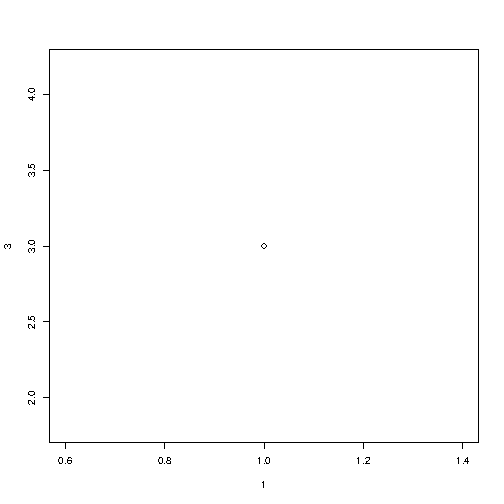
Try it Yourself » To draw more points, use vectors: ExampleDraw two points in the diagram, one at position (1, 3) and one in position (8, 10): plot(c(1, 8), c(3, 10)) Result: 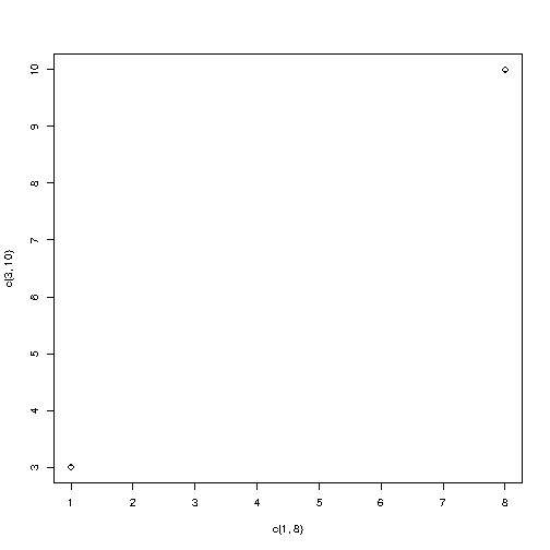
Try it Yourself »
Multiple PointsYou can plot as many points as you like, just make sure you have the same number of points in both axis: Exampleplot(c(1, 2, 3, 4, 5), c(3, 7, 8, 9, 12)) Result: 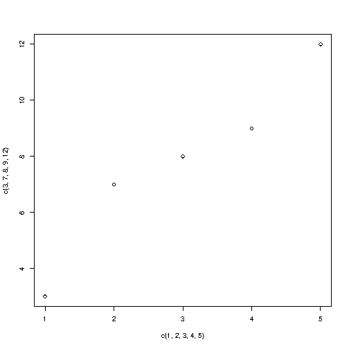
Try it Yourself » For better organization, when you have many values, it is better to use variables: Examplex <- c(1, 2, 3, 4, 5) y <- c(3, 7, 8, 9, 12)
plot(x, y) Result:
Try it Yourself »
Sequences of PointsIf you want to draw dots in a sequence, on both the x-axis and the y-axis, use the : operator: Exampleplot(1:10) Result:
Try it Yourself »
Draw a LineThe plot() function also takes a type parameter with the value l to draw a line to connect all the points in the diagram: Exampleplot(1:10, type="l") Result: 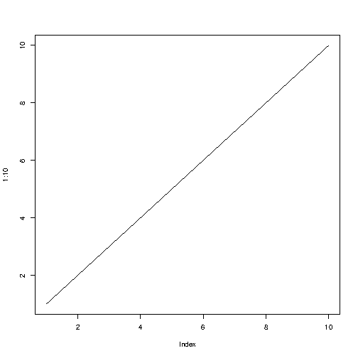
Try it Yourself »
Plot LabelsThe plot() function also accept other parameters, such as main, xlab and ylab if you want to customize the graph with a main title and different labels for the x and y-axis: Exampleplot(1:10, main="My Graph", xlab="The x-axis", ylab="The y axis") Result: 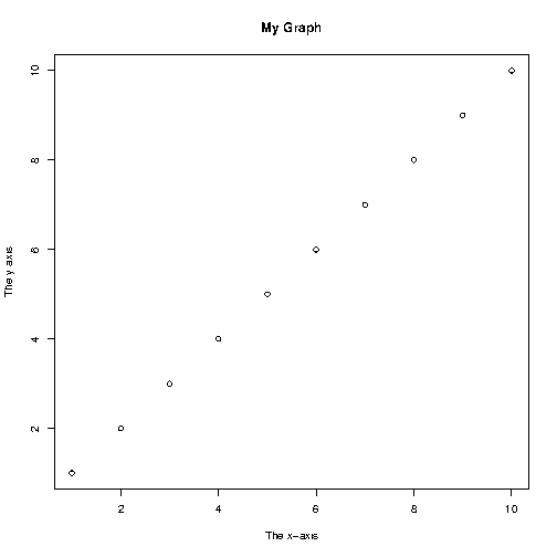
Try it Yourself »
Graph AppearanceThere are many other parameters you can use to change the appearance of the points. ColorsUse col="color" to add a color to the points: Exampleplot(1:10, col="red") Result: 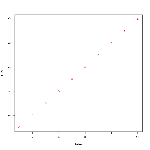
Try it Yourself » SizeUse cex=number to change the size of the points (1 is default, while 0.5 means 50% smaller, and 2 means 100% larger): Exampleplot(1:10, cex=2) Result: 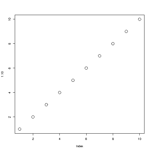
Try it Yourself » Point ShapeUse pch with a value from 0 to 25 to change the point shape format: Exampleplot(1:10, pch=25, cex=2) Result: 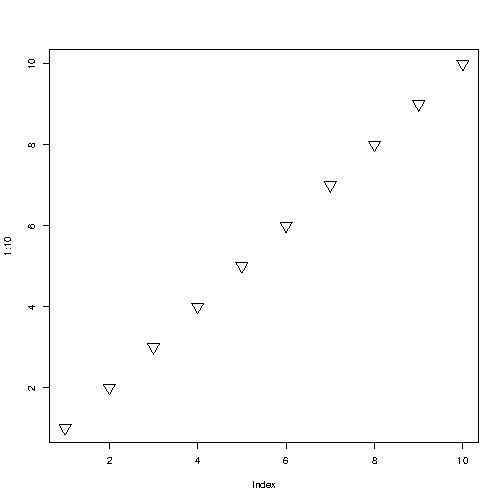
Try it Yourself » The values of the pch parameter ranges from 0 to 25, which means that we can choose up to 26 different types of point shapes: 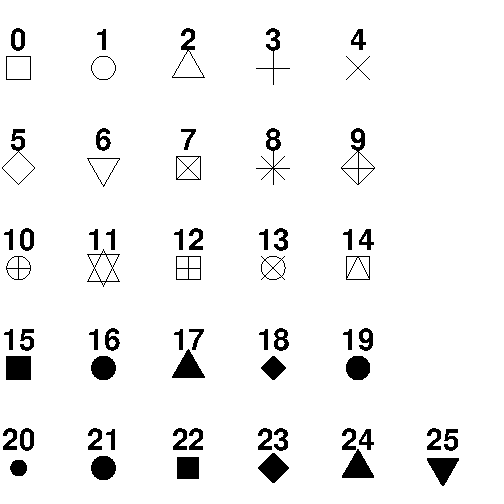
|
| R Line❮ Previous Next ❯
Line GraphsA line graph has a line that connects all the points in a diagram. To create a line, use the plot() function and add the type parameter with a value of "l": Exampleplot(1:10, type="l") Result:
Try it Yourself »
Line ColorThe line color is black by default. To change the color, use the col parameter: Exampleplot(1:10, type="l", col="blue") Result: 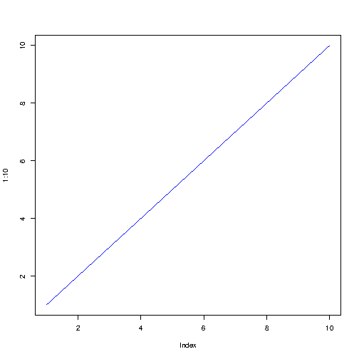
Try it Yourself »
Line WidthTo change the width of the line, use the lwd parameter (1 is default, while 0.5 means 50% smaller, and 2 means 100% larger): Exampleplot(1:10, type="l", lwd=2) Result: 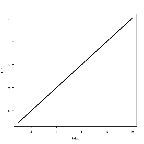
Try it Yourself »
Line StylesThe line is solid by default. Use the lty parameter with a value from 0 to 6 to specify the line format. For example, lty=3 will display a dotted line instead of a solid line: Exampleplot(1:10, type="l", lwd=5, lty=3) Result: 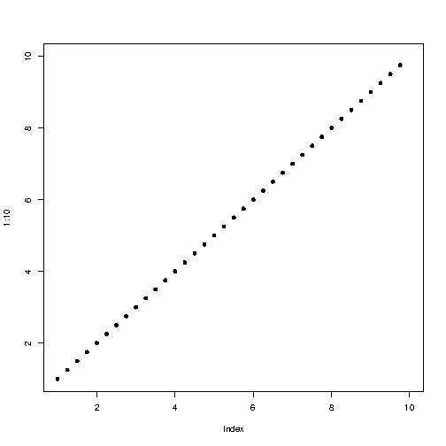
Try it Yourself » Available parameter values for lty: - 0 removes the line
- 1 displays a solid line
- 2 displays a dashed line
- 3 displays a dotted line
- 4 displays a "dot dashed" line
- 5 displays a "long dashed" line
- 6 displays a "two dashed" line
Multiple LinesTo display more than one line in a graph, use the plot() function together with the lines() function: Exampleline1 <- c(1,2,3,4,5,10) line2 <- c(2,5,7,8,9,10)
plot(line1, type = "l", col = "blue") lines(line2, type="l", col = "red") Result: 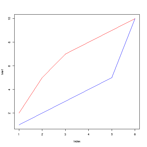
Try it Yourself » |
| R Scatter Plot❮ Previous Next ❯
Scatter PlotsYou learned from the Plot chapter that the plot() function is used to plot numbers against each other. A "scatter plot" is a type of plot used to display the relationship between two numerical variables, and plots one dot for each observation. It needs two vectors of same length, one for the x-axis (horizontal) and one for the y-axis (vertical): Examplex <- c(5,7,8,7,2,2,9,4,11,12,9,6) y <- c(99,86,87,88,111,103,87,94,78,77,85,86)
plot(x, y) Result: 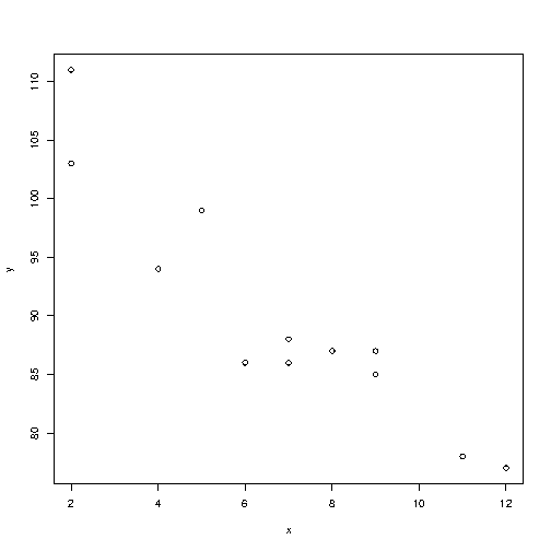
Try it Yourself » The observation in the example above should show the result of 12 cars passing by. That might not be clear for someone who sees the graph for the first time, so let's add a header and different labels to describe the scatter plot better: Examplex <- c(5,7,8,7,2,2,9,4,11,12,9,6) y <- c(99,86,87,88,111,103,87,94,78,77,85,86)
plot(x, y, main="Observation of Cars", xlab="Car age", ylab="Car speed") Result: 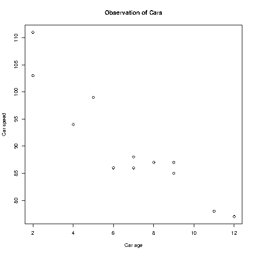
Try it Yourself » To recap, the observation in the example above is the result of 12 cars passing by. The x-axis shows how old the car is. The y-axis shows the speed of the car when it passes. Are there any relationships between the observations? It seems that the newer the car, the faster it drives, but that could be a coincidence, after all we only registered 12 cars.
Compare PlotsIn the example above, there seems to be a relationship between the car speed and age, but what if we plot the observations from another day as well? Will the scatter plot tell us something else? To compare the plot with another plot, use the points() function: ExampleDraw two plots on the same figure: # day one, the age and speed of 12 cars: x1 <- c(5,7,8,7,2,2,9,4,11,12,9,6) y1 <- c(99,86,87,88,111,103,87,94,78,77,85,86)
# day two, the age and speed of 15 cars: x2 <- c(2,2,8,1,15,8,12,9,7,3,11,4,7,14,12) y2 <- c(100,105,84,105,90,99,90,95,94,100,79,112,91,80,85)
plot(x1, y1, main="Observation of Cars", xlab="Car age", ylab="Car speed", col="red", cex=2) points(x2, y2, col="blue", cex=2) Result: 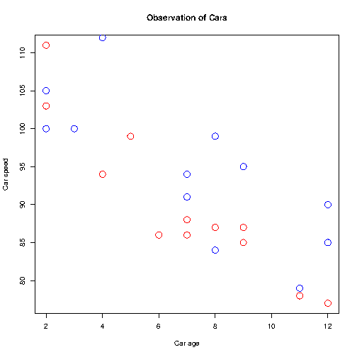
Try it Yourself » Note: To be able to see the difference of the comparison, you must assign different colors to the plots (by using the col parameter). Red represents the values of day 1, while blue represents day 2. Note that we have also added the cex parameter to increase the size of the dots. Conclusion of observation: By comparing the two plots, I think it is safe to say that they both gives us the same conclusion: the newer the car, the faster it drives.
❮ Previous Next ❯
|
| R Pie Charts❮ Previous Next ❯
Pie ChartsA pie chart is a circular graphical view of data. Use the pie() function to draw pie charts: Example# Create a vector of pies x <- c(10,20,30,40)
# Display the pie chart pie(x) Result: 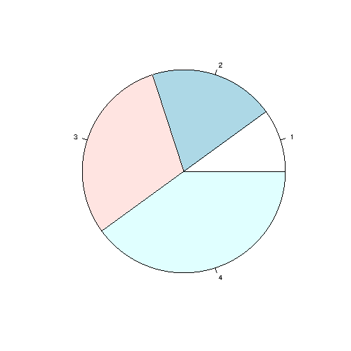
Try it Yourself » Example ExplainedAs you can see the pie chart draws one pie for each value in the vector (in this case 10, 20, 30, 40). By default, the plotting of the first pie starts from the x-axis and move counterclockwise. Note: The size of each pie is determined by comparing the value with all the other values, by using this formula: The value divided by the sum of all values: x/sum(x)
Start AngleYou can change the start angle of the pie chart with the init.angle parameter. The value of init.angle is defined with angle in degrees, where default angle is 0. ExampleStart the first pie at 90 degrees: # Create a vector of pies x <- c(10,20,30,40)
# Display the pie chart and start the first pie at 90 degrees pie(x, init.angle = 90) Result: 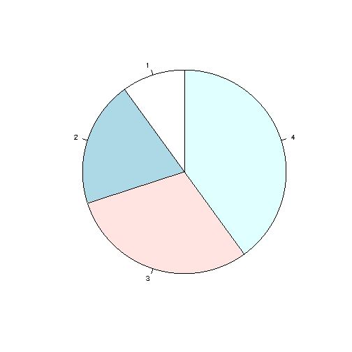
Try it Yourself »
Labels and HeaderUse the label parameter to add a label to the pie chart, and use the main parameter to add a header: Example# Create a vector of pies x <- c(10,20,30,40)
# Create a vector of labels mylabel <- c("Apples", "Bananas", "Cherries", "Dates")
# Display the pie chart with labels pie(x, label = mylabel, main = "Fruits") Result: 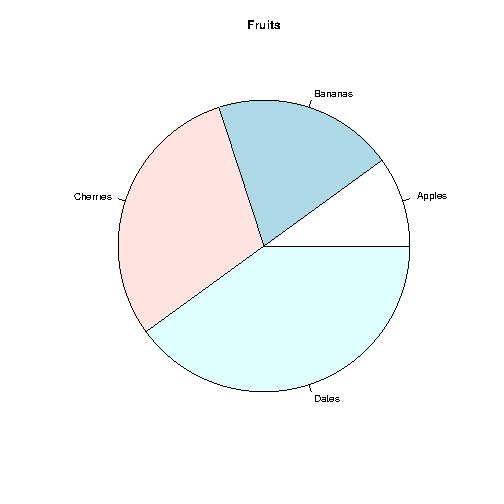
Try it Yourself »
ColorsYou can add a color to each pie with the col parameter: Example# Create a vector of colors colors <- c("blue", "yellow", "green", "black")
# Display the pie chart with colors pie(x, label = mylabel, main = "Fruits", col = colors) Result: 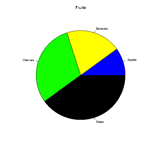
Try it Yourself »
LegendTo add a list of explanation for each pie, use the legend() function: Example# Create a vector of labels mylabel <- c("Apples", "Bananas", "Cherries", "Dates")
# Create a vector of colors colors <- c("blue", "yellow", "green", "black")
# Display the pie chart with colors pie(x, label = mylabel, main = "Pie Chart", col = colors)
# Display the explanation box legend("bottomright", mylabel, fill = colors) Result: 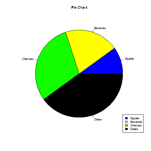
Try it Yourself » The legend can be positioned as either: bottomright, bottom, bottomleft, left, topleft, top, topright, right, center
|
| R Bar Charts❮ Previous Next ❯
Bar ChartsA bar chart uses rectangular bars to visualize data. Bar charts can be displayed horizontally or vertically. The height or length of the bars are proportional to the values they represent. Use the barplot() function to draw a vertical bar chart: Example# x-axis values x <- c("A", "B", "C", "D")
# y-axis values y <- c(2, 4, 6, 8)
barplot(y, names.arg = x) Result: 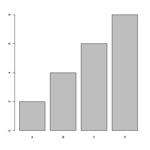
Try it Yourself » Example Explained- The x variable represents values in the x-axis (A,B,C,D)
- The y variable represents values in the y-axis (2,4,6,8)
- Then we use the barplot() function to create a bar chart of the values
- names.arg defines the names of each observation in the x-axis
Bar ColorUse the col parameter to change the color of the bars: Examplex <- c("A", "B", "C", "D") y <- c(2, 4, 6, 8)
barplot(y, names.arg = x, col = "red") Result: 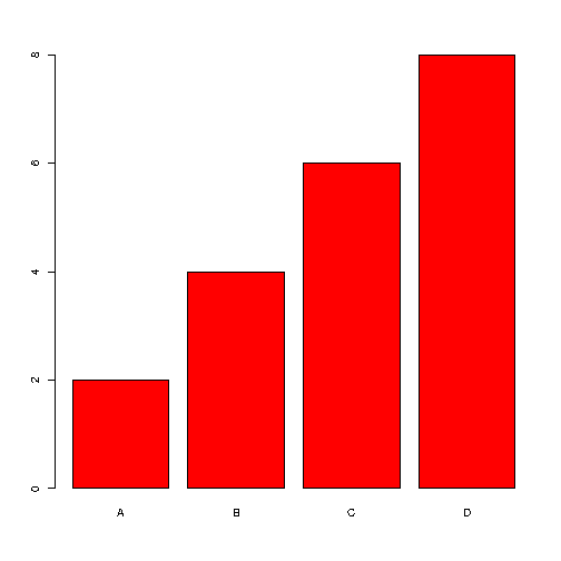
Try it Yourself »
Density / Bar TextureTo change the bar texture, use the density parameter: Examplex <- c("A", "B", "C", "D") y <- c(2, 4, 6, 8)
barplot(y, names.arg = x, density = 10) Result: 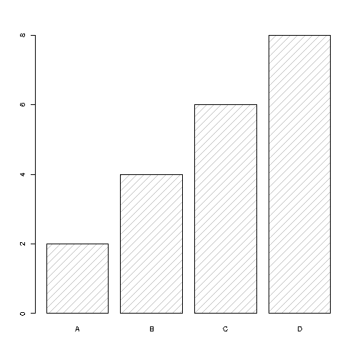
Try it Yourself »
Bar WidthUse the width parameter to change the width of the bars: Examplex <- c("A", "B", "C", "D") y <- c(2, 4, 6, 8)
barplot(y, names.arg = x, width = c(1,2,3,4)) Result: 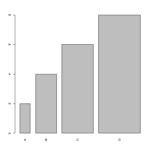
Try it Yourself »
Horizontal BarsIf you want the bars to be displayed horizontally instead of vertically, use horiz=TRUE: Examplex <- c("A", "B", "C", "D") y <- c(2, 4, 6, 8)
barplot(y, names.arg = x, horiz = TRUE) Result: 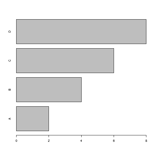
Try it Yourself »
❮ Previous Next ❯
|
|
|
R Statistics |
|
| R Statistics❮ Previous Next ❯
Statistics IntroductionStatistics is the science of analyzing, reviewing and conclude data. Some basic statistical numbers include: - Mean, median and mode
- Minimum and maximum value
- Percentiles
- Variance and Standard Devation
- Covariance and Correlation
- Probability distributions
The R language was developed by two statisticians. It has many built-in functionalities, in addition to libraries for the exact purpose of statistical analysis. You will learn about these features, and how to use them in the next chapters. Tip: If you are completely new to statistics, and want to learn more about it, visit our Statistics Tutorial.
❮ Previous Next ❯
|
| R Data Set❮ Previous Next ❯
Data SetA data set is a collection of data, often presented in a table. There is a popular built-in data set in R called "mtcars" (Motor Trend Car Road Tests), which is retrieved from the 1974 Motor Trend US Magazine. In the examples below (and for the next chapters), we will use the mtcars data set, for statistical purposes: Example# Print the mtcars data set mtcars Result: mpg cyl disp hp drat wt qsec vs am gear carb Mazda RX4 21.0 6 160.0 110 3.90 2.620 16.46 0 1 4 4 Mazda RX4 Wag 21.0 6 160.0 110 3.90 2.875 17.02 0 1 4 4 Datsun 710 22.8 4 108.0 93 3.85 2.320 18.61 1 1 4 1 Hornet 4 Drive 21.4 6 258.0 110 3.08 3.215 19.44 1 0 3 1 Hornet Sportabout 18.7 8 360.0 175 3.15 3.440 17.02 0 0 3 2 Valiant 18.1 6 225.0 105 2.76 3.460 20.22 1 0 3 1 Duster 360 14.3 8 360.0 245 3.21 3.570 15.84 0 0 3 4 Merc 240D 24.4 4 146.7 62 3.69 3.190 20.00 1 0 4 2 Merc 230 22.8 4 140.8 95 3.92 3.150 22.90 1 0 4 2 Merc 280 19.2 6 167.6 123 3.92 3.440 18.30 1 0 4 4 Merc 280C 17.8 6 167.6 123 3.92 3.440 18.90 1 0 4 4 Merc 450SE 16.4 8 275.8 180 3.07 4.070 17.40 0 0 3 3 Merc 450SL 17.3 8 275.8 180 3.07 3.730 17.60 0 0 3 3 Merc 450SLC 15.2 8 275.8 180 3.07 3.780 18.00 0 0 3 3 Cadillac Fleetwood 10.4 8 472.0 205 2.93 5.250 17.98 0 0 3 4 Lincoln Continental 10.4 8 460.0 215 3.00 5.424 17.82 0 0 3 4 Chrysler Imperial 14.7 8 440.0 230 3.23 5.345 17.42 0 0 3 4 Fiat 128 32.4 4 78.7 66 4.08 2.200 19.47 1 1 4 1 Honda Civic 30.4 4 75.7 52 4.93 1.615 18.52 1 1 4 2 Toyota Corolla 33.9 4 71.1 65 4.22 1.835 19.90 1 1 4 1 Toyota Corona 21.5 4 120.1 97 3.70 2.465 20.01 1 0 3 1 Dodge Challenger 15.5 8 318.0 150 2.76 3.520 16.87 0 0 3 2 AMC Javelin 15.2 8 304.0 150 3.15 3.435 17.30 0 0 3 2 Camaro Z28 13.3 8 350.0 245 3.73 3.840 15.41 0 0 3 4 Pontiac Firebird 19.2 8 400.0 175 3.08 3.845 17.05 0 0 3 2 Fiat X1-9 27.3 4 79.0 66 4.08 1.935 18.90 1 1 4 1 Porsche 914-2 26.0 4 120.3 91 4.43 2.140 16.70 0 1 5 2 Lotus Europa 30.4 4 95.1 113 3.77 1.513 16.90 1 1 5 2 Ford Pantera L 15.8 8 351.0 264 4.22 3.170 14.50 0 1 5 4 Ferrari Dino 19.7 6 145.0 175 3.62 2.770 15.50 0 1 5 6 Maserati Bora 15.0 8 301.0 335 3.54 3.570 14.60 0 1 5 8 Volvo 142E 21.4 4 121.0 109 4.11 2.780 18.60 1 1 4 2
Try it Yourself »
Information About the Data SetYou can use the question mark (?) to get information about the mtcars data set: Example# Use the question mark to get information about the data set
?mtcars Result: mtcars {datasets} | R Documentation |
Motor Trend Car Road TestsDescriptionThe data was extracted from the 1974 Motor Trend US magazine, and comprises fuel consumption and 10 aspects of automobile design and performance for 32 automobiles (1973-74 models). Usagemtcars FormatA data frame with 32 observations on 11 (numeric) variables. [, 1] | mpg | Miles/(US) gallon | [, 2] | cyl | Number of cylinders | [, 3] | disp | Displacement (cu.in.) | [, 4] | hp | Gross horsepower | [, 5] | drat | Rear axle ratio | [, 6] | wt | Weight (1000 lbs) | [, 7] | qsec | 1/4 mile time | [, 8] | vs | Engine (0 = V-shaped, 1 = straight) | [, 9] | am | Transmission (0 = automatic, 1 = manual) | [,10] | gear | Number of forward gears | [,11] | carb | Number of carburetors |
NoteHenderson and Velleman (1981) comment in a footnote to Table 1: 'Hocking [original transcriber]'s noncrucial coding of the Mazda's rotary engine as a straight six-cylinder engine and the Porsche's flat engine as a V engine, as well as the inclusion of the diesel Mercedes 240D, have been retained to enable direct comparisons to be made with previous analyses.' SourceHenderson and Velleman (1981), Building multiple regression models interactively. Biometrics, 37, 391-411. Examplesrequire(graphics) pairs(mtcars, main = "mtcars data", gap = 1/4) coplot(mpg ~ disp | as.factor(cyl), data = mtcars, panel = panel.smooth, rows = 1) ## possibly more meaningful, e.g., for summary() or bivariate plots: mtcars2 <- within(mtcars, { vs <- factor(vs, labels = c("V", "S")) am <- factor(am, labels = c("automatic", "manual")) cyl <- ordered(cyl) gear <- ordered(gear) carb <- ordered(carb) }) summary(mtcars2)
Try it Yourself »
Get InformationUse the dim() function to find the dimensions of the data set, and the names() function to view the names of the variables: ExampleData_Cars <- mtcars # create a variable of the mtcars data set for better organization
# Use dim() to find the dimension of the data set dim(Data_Cars)
# Use names() to find the names of the variables from the data set names(Data_Cars) Result: [1] 32 11 [1] "mpg" "cyl" "disp" "hp" "drat" "wt" "qsec" "vs" "am" "gear" [11] "carb"
Try it Yourself » Use the rownames() function to get the name of each row in the first column, which is the name of each car: ExampleData_Cars <- mtcars
rownames(Data_Cars) Result: [1] "Mazda RX4" "Mazda RX4 Wag" "Datsun 710" [4] "Hornet 4 Drive" "Hornet Sportabout" "Valiant" [7] "Duster 360" "Merc 240D" "Merc 230" [10] "Merc 280" "Merc 280C" "Merc 450SE" [13] "Merc 450SL" "Merc 450SLC" "Cadillac Fleetwood" [16] "Lincoln Continental" "Chrysler Imperial" "Fiat 128" [19] "Honda Civic" "Toyota Corolla" "Toyota Corona" [22] "Dodge Challenger" "AMC Javelin" "Camaro Z28" [25] "Pontiac Firebird" "Fiat X1-9" "Porsche 914-2" [28] "Lotus Europa" "Ford Pantera L" "Ferrari Dino" [31] "Maserati Bora" "Volvo 142E" Try it Yourself » From the examples above, we have found out that the data set has 32 observations (Mazda RX4, Mazda RX4 Wag, Datsun 710, etc) and 11 variables (mpg, cyl, disp, etc). A variable is defined as something that can be measured or counted. Here is a brief explanation of the variables from the mtcars data set: Variable Name | Description | mpg | Miles/(US) Gallon | cyl | Number of cylinders | disp | Displacement | hp | Gross horsepower | drat | Rear axle ratio | wt | Weight (1000 lbs) | qsec | 1/4 mile time | vs | Engine (0 = V-shaped, 1 = straight) | am | Transmission (0 = automatic, 1 = manual) | gear | Number of forward gears | carb | Number of carburetors |
Print Variable ValuesIf you want to print all values that belong to a variable, access the data frame by using the $ sign, and the name of the variable (for example cyl (cylinders)): ExampleData_Cars <- mtcars
Data_Cars$cyl Result: [1] 6 6 4 6 8 6 8 4 4 6 6 8 8 8 8 8 8 4 4 4 4 8 8 8 8 4 4 4 8 6 8 4 Try it Yourself »
Sort Variable ValuesTo sort the values, use the sort() function: ExampleData_Cars <- mtcars
sort(Data_Cars$cyl) Result: [1] 4 4 4 4 4 4 4 4 4 4 4 6 6 6 6 6 6 6 8 8 8 8 8 8 8 8 8 8 8 8 8 8 Try it Yourself » From the examples above, we see that most cars have 4 and 8 cylinders.
Analyzing the DataNow that we have some information about the data set, we can start to analyze it with some statistical numbers. For example, we can use the summary() function to get a statistical summary of the data: ExampleData_Cars <- mtcars
summary(Data_Cars) Try it Yourself » Do not worry if you do not understand the output numbers. You will master them shortly. The summary() function returns six statistical numbers for each variable: - Min
- First quantile (percentile)
- Median
- Mean
- Third quantile (percentile)
- Max
We will cover all of them, along with other statistical numbers in the next chapters.
❮ Previous Next ❯ |
| R Max and Min❮ Previous Next ❯
Max MinIn the previous chapter, we introduced the mtcars data set. We will continue to use this data set throughout the next pages. You learned from the R Math chapter that R has several built-in math functions. For example, the min() and max() functions can be used to find the lowest or highest value in a set: ExampleFind the largest and smallest value of the variable hp (horsepower). Data_Cars <- mtcars
max(Data_Cars$hp) min(Data_Cars$hp) Result: [1] 335 [1] 52 Try it Yourself » Now we know that the largest horsepower value in the set is 335, and the lowest 52. We could take a look at the data set and try to find out which car these two values belongs to: Observation of cars mpg cyl disp hp drat wt qsec vs am gear carb Mazda RX4 21.0 6 160.0 110 3.90 2.620 16.46 0 1 4 4 Mazda RX4 Wag 21.0 6 160.0 110 3.90 2.875 17.02 0 1 4 4 Datsun 710 22.8 4 108.0 93 3.85 2.320 18.61 1 1 4 1 Hornet 4 Drive 21.4 6 258.0 110 3.08 3.215 19.44 1 0 3 1 Hornet Sportabout 18.7 8 360.0 175 3.15 3.440 17.02 0 0 3 2 Valiant 18.1 6 225.0 105 2.76 3.460 20.22 1 0 3 1 Duster 360 14.3 8 360.0 245 3.21 3.570 15.84 0 0 3 4 Merc 240D 24.4 4 146.7 62 3.69 3.190 20.00 1 0 4 2 Merc 230 22.8 4 140.8 95 3.92 3.150 22.90 1 0 4 2 Merc 280 19.2 6 167.6 123 3.92 3.440 18.30 1 0 4 4 Merc 280C 17.8 6 167.6 123 3.92 3.440 18.90 1 0 4 4 Merc 450SE 16.4 8 275.8 180 3.07 4.070 17.40 0 0 3 3 Merc 450SL 17.3 8 275.8 180 3.07 3.730 17.60 0 0 3 3 Merc 450SLC 15.2 8 275.8 180 3.07 3.780 18.00 0 0 3 3 Cadillac Fleetwood 10.4 8 472.0 205 2.93 5.250 17.98 0 0 3 4 Lincoln Continental 10.4 8 460.0 215 3.00 5.424 17.82 0 0 3 4 Chrysler Imperial 14.7 8 440.0 230 3.23 5.345 17.42 0 0 3 4 Fiat 128 32.4 4 78.7 66 4.08 2.200 19.47 1 1 4 1 Honda Civic 30.4 4 75.7 52 4.93 1.615 18.52 1 1 4 2 Toyota Corolla 33.9 4 71.1 65 4.22 1.835 19.90 1 1 4 1 Toyota Corona 21.5 4 120.1 97 3.70 2.465 20.01 1 0 3 1 Dodge Challenger 15.5 8 318.0 150 2.76 3.520 16.87 0 0 3 2 AMC Javelin 15.2 8 304.0 150 3.15 3.435 17.30 0 0 3 2 Camaro Z28 13.3 8 350.0 245 3.73 3.840 15.41 0 0 3 4 Pontiac Firebird 19.2 8 400.0 175 3.08 3.845 17.05 0 0 3 2 Fiat X1-9 27.3 4 79.0 66 4.08 1.935 18.90 1 1 4 1 Porsche 914-2 26.0 4 120.3 91 4.43 2.140 16.70 0 1 5 2 Lotus Europa 30.4 4 95.1 113 3.77 1.513 16.90 1 1 5 2 Ford Pantera L 15.8 8 351.0 264 4.22 3.170 14.50 0 1 5 4 Ferrari Dino 19.7 6 145.0 175 3.62 2.770 15.50 0 1 5 6 Maserati Bora 15.0 8 301.0 335 3.54 3.570 14.60 0 1 5 8 Volvo 142E 21.4 4 121.0 109 4.11 2.780 18.60 1 1 4 2
By observing the table, it looks like the largest hp value belongs to a Maserati Bora, and the lowest belongs to a Honda Civic. However, it is much easier (and safer) to let R find out this for us. For example, we can use the which.max() and which.min() functions to find the index position of the max and min value in the table: ExampleData_Cars <- mtcars
which.max(Data_Cars$hp) which.min(Data_Cars$hp) Result: [1] 31 [1] 19 Try it Yourself » Or even better, combine which.max() and which.min() with the rownames() function to get the name of the car with the largest and smallest horsepower: ExampleData_Cars <- mtcars
rownames(Data_Cars)[which.max(Data_Cars$hp)] rownames(Data_Cars)[which.min(Data_Cars$hp)] Result: [1] "Maserati Bora" [1] "Honda Civic" Try it Yourself » Now we know for sure:
Maserati Bora is the car with the highest horsepower, and Honda Civic is the car with the lowest horsepower.
OutliersMax and min can also be used to detect outliers. An outlier is a data point that differs from rest of the observations. Example of data points that could have been outliers in the mtcars data set: - If maximum of forward gears of a car was 11
- If minimum of horsepower of a car was 0
- If maximum weight of a car was 50 000 lbs
❮ Previous Next ❯ |
| R Mean❮ Previous Next ❯
Mean, Median, and ModeIn statistics, there are often three values that interests us: - Mean - The average value
- Median - The middle value
- Mode - The most common value
MeanTo calculate the average value (mean) of a variable from the mtcars data set, find the sum of all values, and divide the sum by the number of values. Sorted observation of wt (weight)1.513 | 1.615 | 1.835 | 1.935 | 2.140 | 2.200 | 2.320 | 2.465 | 2.620 | 2.770 | 2.780 | 2.875 | 3.150 | 3.170 | 3.190 | 3.215 | 3.435 | 3.440 | 3.440 | 3.440 | 3.460 | 3.520 | 3.570 | 3.570 | 3.730 | 3.780 | 3.840 | 3.845 | 4.070 | 5.250 | 5.345 | 5.424 |
Luckily for us, the mean() function in R can do it for you: ExampleFind the average weight (wt) of a car: Data_Cars <- mtcars
mean(Data_Cars$wt) Result: [1] 3.21725 Try it Yourself »
❮ Previous Next ❯
|
| R MedianMedianThe median value is the value in the middle, after you have sorted all the values. If we take a look at the values of the wt variable (from the mtcars data set), we will see that there are two numbers in the middle: Sorted observation of wt (weight)1.513 | 1.615 | 1.835 | 1.935 | 2.140 | 2.200 | 2.320 | 2.465 | 2.620 | 2.770 | 2.780 | 2.875 | 3.150 | 3.170 | 3.190 | 3.215 | 3.435 | 3.440 | 3.440 | 3.440 | 3.460 | 3.520 | 3.570 | 3.570 | 3.730 | 3.780 | 3.840 | 3.845 | 4.070 | 5.250 | 5.345 | 5.424 |
Note: If there are two numbers in the middle, you must divide the sum of those numbers by two, to find the median. Luckily, R has a function that does all of that for you: Just use the median() function to find the middle value: ExampleFind the mid point value of weight (wt): Data_Cars <- mtcars
median(Data_Cars$wt) Result: [1] 3.325 Try it Yourself »
|
| R ModeModeThe mode value is the value that appears the most number of times.R does not have a function to calculate the mode. However, we can create our own function to find it. If we take a look at the values of the wt variable (from the mtcars data set), we will see that the numbers 3.440 are often shown: Sorted observation of wt (weight)1.513 | 1.615 | 1.835 | 1.935 | 2.140 | 2.200 | 2.320 | 2.465 | 2.620 | 2.770 | 2.780 | 2.875 | 3.150 | 3.170 | 3.190 | 3.215 | 3.435 | 3.440 | 3.440 | 3.440 | 3.460 | 3.520 | 3.570 | 3.570 | 3.730 | 3.780 | 3.840 | 3.845 | 4.070 | 5.250 | 5.345 | 5.424 |
Instead of counting it ourselves, we can use the following code to find the mode: ExampleData_Cars <- mtcars
names(sort(-table(Data_Cars$wt)))[1] Result: [1] "3.44" Try it Yourself » From the example above, we now know that the number that appears the most number of times in mtcars wt variable is 3.44 or 3.440 lbs. |
| R Percentiles❮ Previous Next ❯
PercentilesPercentiles are used in statistics to give you a number that describes the value that a given percent of the values are lower than. If we take a look at the values of the wt (weight) variable from the mtcars data set: Observation of wt (weight)1.513 | 1.615 | 1.835 | 1.935 | 2.140 | 2.200 | 2.320 | 2.465 | 2.620 | 2.770 | 2.780 | 2.875 | 3.150 | 3.170 | 3.190 | 3.215 | 3.435 | 3.440 | 3.440 | 3.440 | 3.460 | 3.520 | 3.570 | 3.570 | 3.730 | 3.780 | 3.840 | 3.845 | 4.070 | 5.250 | 5.345 | 5.424 |
What is the 75. percentile of the weight of the cars? The answer is 3.61 or 3 610 lbs, meaning that 75% or the cars weight 3 610 lbs or less: ExampleData_Cars <- mtcars
# c() specifies which percentile you want quantile(Data_Cars$wt, c(0.75)) Result: 75% 3.61 Try it Yourself » If you run the quantile() function without specifying the c() parameter, you will get the percentiles of 0, 25, 50, 75 and 100: ExampleData_Cars <- mtcars
quantile(Data_Cars$wt) Result: 0% 25% 50% 75% 100% 1.51300 2.58125 3.32500 3.61000 5.42400
Try it Yourself »
QuartilesQuartiles are data divided into four parts, when sorted in an ascending order: - The value of the first quartile cuts off the first 25% of the data
- The value of the second quartile cuts off the first 50% of the data
- The value of the third quartile cuts off the first 75% of the data
- The value of the fourth quartile cuts off the 100% of the data
Use the quantile() function to get the quartiles.
❮ Previous Next ❯ |
|
|
R Examples |
|
|
|
|
|